This page lists LAMMPS performance on several benchmark problems, run on various machines, both in serial and parallel and on GPUs. Note that input and sample output files for many of these benchmark tests are provided in the bench directory of the LAMMPS distribution. See the bench/README file for details.
Note that most of these numbers are quite old and thus do not reflect numbers that can be achieved with current hardware or what kind of improvements have been added to the LAMMPS code since then. They do, however, still represent the relative strong and weak scaling behavior in most cases.
Thanks to the following individuals for running the various benchmarks:
These are the parallel machines for which benchmark data is given for the CPU benchmarks below. See the Kokkos, Intel, and GPU sections for machine specifications for those GPU and Phi platforms.
The "Processors" column is the most number of processors on that machine that LAMMPS was run on. Message passing bandwidth and latency is in units of Mb/sec and microsecs at the MPI level, i.e. what a program like LAMMPS sees. More information on machine characteristics, including their "birth" year, is given at the bottom of the page.
| Vendor/Machine | Processors | Site | CPU | Interconnect | Bandwidth | Latency |
| Dell T7500 dual hex-core desktop | 12 | SNL | 3.47 GHz Xeon | on-chip | ?? | ?? |
| Xeon/Myrinet cluster | 512 | SNL | 3.4 GHz dual Xeons (64-bit) | Myrinet | 230 | 9 |
| IBM p690+ | 512 | Daresbury | 1.7 GHz Power4+ | custom | 1450 | 6 |
| IBM BG/L | 65536 | LLNL | 700 MHz PowerPC 440 | custom | 150 | 3 |
| Cray XT3 | 10000 | SNL | 2.0 GHz Opteron | Cstar | 1100 | 7 |
| Cray XT5 | 1920 | SNL | 2.4 GHz Opteron | Cstar | 1100 | 7 |
One-processor timings are also listed for some older machines whose characteristics are also given below.
| Name | Machine | Processors | Site | CPU | Interconnect | Bandwidth | Latency |
| Laptop | Mac PowerBook | 1 | SNL | 1 GHz G4 PowerPC | N/A | N/A | N/A |
| ASCI Red | Intel | 1500 | SNL | 333 MHz Pentium III | custom | 310 | 18 |
| Ross | custom Linux cluster | 64 | SNL | 500 MHz DEC Alpha | Myrinet | 100 | 65 |
| Liberty | HP Linux cluster | 64 | SNL | 3.0 GHz dual Xeons (32-bit) | Myrinet | 230 | 9 |
| Cheetah | IBM p690 | 64 | ORNL | 1.3 GHz Power4 | custom | 1490 | 7 |
Billion-atom LJ timings are also given for GPU clusters, with more characteristics given below.
| Name | Machine | GPUs | Site | GPU | Interconnect | Bandwidth | Latency |
| Keeneland | Intel/NVIDIA cluster | 360 | ORNL | Tesla M2090 | Qlogic QDR | ??? | ??? |
| Lincoln | Intel/NVIDIA cluster | 384 | NCSA | Tesla C1060 | Infiniband | 1500 | 12 |
For each of the 5 benchmarks, fixed- and scaled-size timings are shown in tables and in comparative plots. Fixed-size means that the same problem with 32,000 atoms was run on varying numbers of processors. Scaled-size means that when run on P processors, the number of atoms in the simulation was P times larger than the one-processor run. Thus a scaled-size 64-processor run is for 2,048,000 atoms; a 32K proc run is for ~1 billion atoms.
All listed CPU times are in seconds for 100 timesteps. Parallel efficiencies refer to the ratio of ideal to actual run time. For example, if perfect speed-up would have given a run-time of 10 seconds, and the actual run time was 12 seconds, then the efficiency is 10/12 or 83.3%. In most cases parallel runs were made on production machines while other jobs were running, which can sometimes degrade performance.
The files needed to run these benchmarks are part of the LAMMPS distribution. If your platform is sufficiently different from the machines listed, you can send your timing results and machine info and we'll add them to this page. Note that the CPU time (in seconds) for a run is what appears in the "Loop time" line of the output log file, e.g.
Loop time of 3.89418 on 8 procs for 100 steps with 32000 atoms
These benchmarks are meant to span a range of simulation styles and computational expense for interaction forces. Since LAMMPS run time scales roughly linearly in the number of atoms simulated, you can use the timing and parallel efficiency data to estimate the CPU cost for problems you want to run on a given number of processors. As the data below illustrates, fixed-size problems generally have parallel efficiencies of 50% or better so long as the atoms/processor is a few hundred or more. Scaled-size problems generally have parallel efficiencies of 80% or more across a wide range of processor counts.
This is a summary of single-processor LAMMPS performance in CPU secs per atom per timestep for the 5 benchmark problems which follow. This is on a Dell Precision T7500 desktop Red Hat linux box with dual hex-core 3.47 GHz Intel Xeon processors, using the Intel 11.1 icc compiler. The ratios indicate that if the atomic LJ system has a normalized cost of 1.0, the bead-spring chains and granular systems run 2x and 4x faster, while the EAM metal and solvated protein models run 2.6x and 16x slower respectively. These differences are primarily due to the expense of computing a particular pairwise force field for a given number of neighbors per atom.
| Problem: | LJ | Chain | EAM | Chute | Rhodopsin |
| CPU/atom/step: | 7.02E-7 | 3.15E-7 | 1.85E-6 | 1.71E-7 | 1.14E-5 |
| Ratio to LJ: | 1.0 | 0.45 | 2.64 | 0.24 | 16.2 |
Input script for this problem.
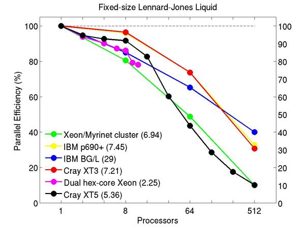
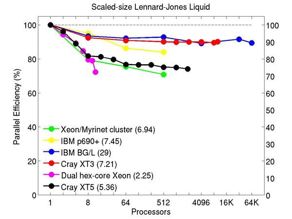
Atomic fluid:
Performance data:
These plots show fixed-size parallel efficiency for the same 32K atom problem run on different numbers of processors and scaled-size efficiency for runs with 32K atoms/proc. Thus a scaled-size 64-processor run is for 2,048,000 atoms; a 32K proc run is for ~1 billion atoms. Each curve is normalized to be 100% on one processor for the respective machine; one-processor timings are shown in parenthesis. Click on the plot for a larger version.
Input script for this problem.
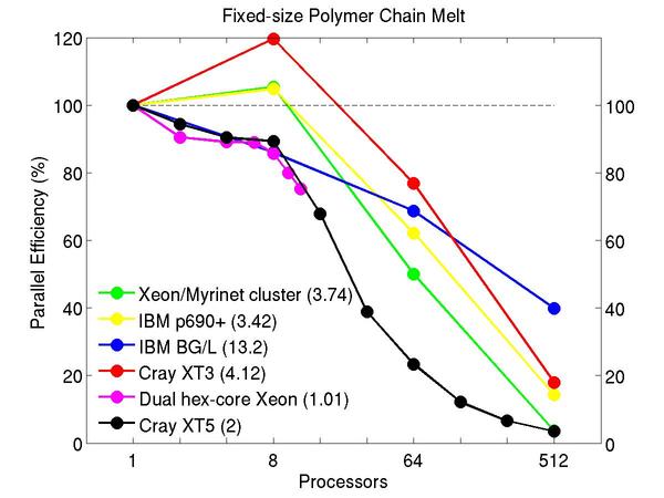
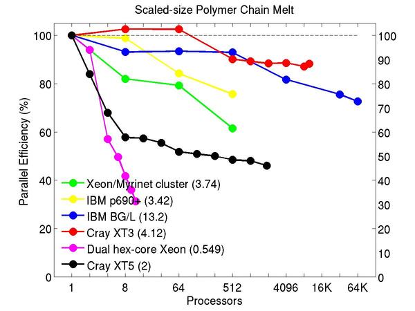
Bead-spring polymer melt with 100-mer chains and FENE bonds:
Performance data:
These plots show fixed-size parallel efficiency for the same 32K atom problem run on different numbers of processors and scaled-size efficiency for runs with 32K atoms/proc. Thus a scaled-size 64-processor run is for 2,048,000 atoms; a 32K proc run is for ~1 billion atoms. Each curve is normalized to be 100% on one processor for the respective machine; one-processor timings are shown in parenthesis. Click on the plot for a larger version.
Input script for this problem.
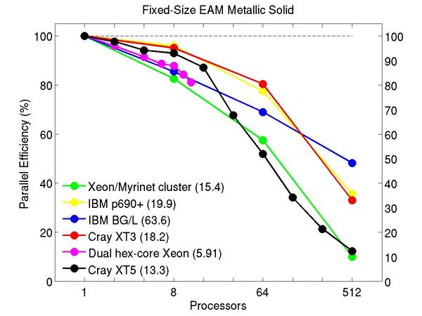
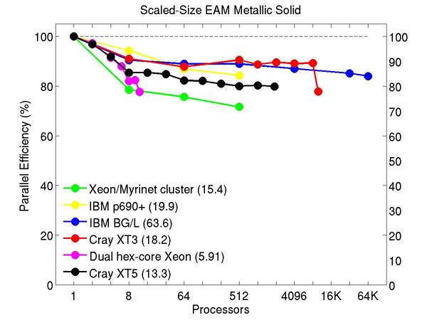
Cu metallic solid with embedded atom method (EAM) potential:
Performance data:
These plots show fixed-size parallel efficiency for the same 32K atom problem run on different numbers of processors and scaled-size efficiency for runs with 32K atoms/proc. Thus a scaled-size 64-processor run is for 2,048,000 atoms; a 32K proc run is for ~1 billion atoms. Each curve is normalized to be 100% on one processor for the respective machine; one-processor timings are shown in parenthesis. Click on the plot for a larger version.
Input script for this problem.
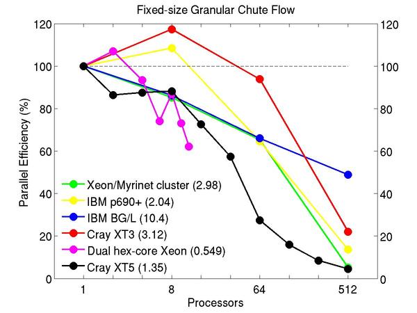
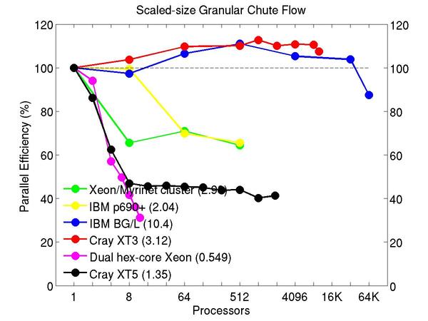
Chute flow of packed granular particles with frictional history potential:
Performance data:
These plots show fixed-size parallel efficiency for the same 32K atom problem run on different numbers of processors and scaled-size efficiency for runs with 32K atoms/proc. Thus a scaled-size 64-processor run is for 2,048,000 atoms; a 32K proc run is for ~1 billion atoms. Each curve is normalized to be 100% on one processor for the respective machine; one-processor timings are shown in parenthesis. Click on the plot for a larger version.
Input script for this problem.
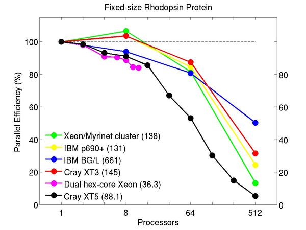
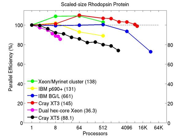
All-atom rhodopsin protein in solvated lipid bilayer with CHARMM force field, long-range Coulombics via PPPM (particle-particle particle mesh), SHAKE constraints. This model contains counter-ions and a reduced amount of water to make a 32K atom system:
Performance data:
These plots show fixed-size parallel efficiency for the same 32K atom problem run on different numbers of processors and scaled-size efficiency for runs with 32K atoms/proc. Thus a scaled-size 64-processor run is for 2,048,000 atoms; a 32K proc run is for ~1 billion atoms. Each curve is normalized to be 100% on one processor for the respective machine; one-processor timings are shown in parenthesis. Click on the plot for a larger version.
Benchmark of the Lennard-Jones potential: /src/USER-INTEL/TEST/in.intel.lj, run using "-v m 0.1". On Sandy Bridge CPU and KNL, "atom_modify sort 100 2.8" was added to the input script.
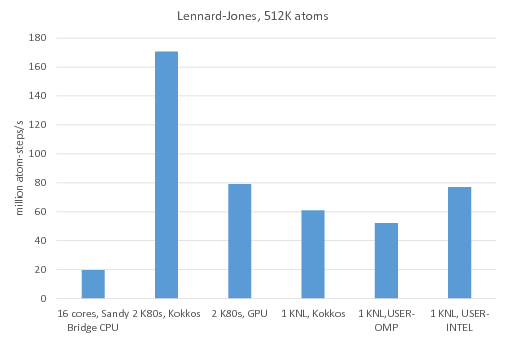
Legend:
16 cores, Sandy Bridge CPU: no accelerator package, 1MPI task per core = 16 MPI tasks total
2 K80 GPUs, Kokkos: Kokkos package used 1 MPI task per internal K80 GPU = 4 MPI tasks total, running on 4 Sandy Bridge CPU cores, full neighbor list, newton off, neighbor list binsize = 2.8
2 K80 GPUs, GPU: GPU package used 4 MPI tasks per internal K80 GPU = 16 MPI tasks total running on 16 Sandy Bridge CPU cores
1 KNL, Kokkos: Kokkos package used 64 MPI tasks x 4 hyperthreads x 4 OpenMP threads, full neighbor list, newton off
1 KNL, USER-OMP: USER-OMP package used 64 MPI tasks x 4 hyperthreads x 4 OpenMP threads
1 KNL, USER-INTEL: USER-INTEL package used 64 MPI tasks x 2 hyperthreads x 2 OpenMP threads
Benchmark of the Stillinger-Weber potential: /src/USER-INTEL/TEST/in.intel.sw, run using "-v m 0.1". For KNL, "atom_modify sort 100 4.77" was added to the input script.
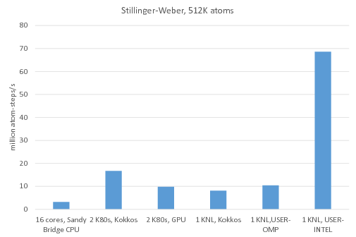
Legend:
16 cores, Sandy Bridge CPU: no accelerator package, 1MPI task per core = 16 MPI tasks total
2 K80 GPUs, Kokkos: Kokkos package used 1 MPI task per internal K80 GPU = 4 MPI tasks total running on 4 Sandy Bridge CPU cores, half neighbor list, newton on
2 K80 GPUs, GPU: GPU package used 4 MPI tasks per internal K80 GPU = 16 MPI tasks total, running on 16 Sandy Bridge CPU cores
1 KNL, Kokkos: Kokkos package used 64 MPI tasks x 4 hyperthreads x 4 OpenMP threads, half neighbor list, newton on
1 KNL, USER-OMP: USER-OMP package used 64 MPI tasks x 4 hyperthreads x 4 OpenMP threads
1 KNL, USER-INTEL: USER-INTEL package used 64 MPI tasks x 4 hyperthreads x 4 OpenMP threads
Benchmark of the Tersoff potential: /src/USER-INTEL/TEST/in.intel.tersoff, was run using "-v m 0.2". For KNL, "atom_modify sort 100 4.2" was added to the input script.
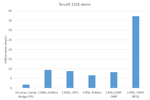
Legend:
16 cores, Sandy Bridge CPU: no accelerator package, 1MPI task per core = 16 MPI tasks total
2 K80 GPUs, Kokkos: Kokkos package used 1 MPI task per internal K80 GPU = 4 MPI tasks total, running on 4 Sandy Bridge CPU cores, half neighbor list, newton on
2 K80 GPUs, GPU: GPU package used 4 MPI tasks per internal K80 GPU = 16 MPI tasks total, running on 16 Sandy Bridge CPU cores
1 KNL, Kokkos: Kokkos package used 64 MPI tasks x 4 hyperthreads x 4 OpenMP threads, half neighbor list, newton on
1 KNL, USER-OMP: USER-OMP package used 64 MPI tasks x 4 hyperthreads x 4 OpenMP threads
1 KNL, USER-INTEL: USER-INTEL package used 64 MPI tasks x 4 hyperthreads x 4 OpenMP threads
This section benchmarks all the accelerator packages available in LAMMPS on the same machine: GPU, KOKKOS, OPT, USER-CUDA, USER-INTEL, USER-OMP. Unaccelerated runs (using the standard LAMMPS styles) are also included for reference.
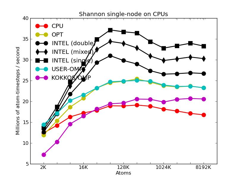
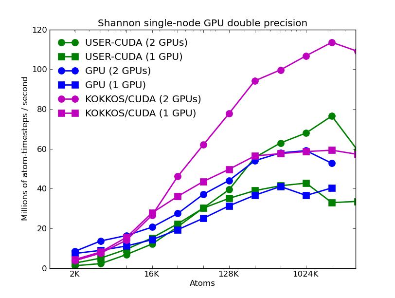
This section shows performance results for a GPU cluster at Sandia National Labs called "shannon". It has 32 nodes, each with two 8-core Sandy Bridge Xeon CPUs (E5-2670, 2.6GHz, HT deactivated), for a total of 512 cores. Twenty-four of the nodes have two NVIDIA Kepler GPUs (K20x, 2688 732 MHz cores). LAMMPS was compiled with the Intel icc compiler, using module openmpi/1.8.1/intel/13.1.SP1.106/cuda/6.0.37.
The benchmark problems themselves are described in more detail above in the CPU section. The input scripts and instructions for running these test cases are included in the bench/KEPLER directory of the LAMMPS distribution.
The first set of 5 plots are for running problmes of various sizes (2K to 8192K atoms) on a single node (16 cores, 1 or 2 GPUs). Note that the y-axis scale is not the same in the various plots. Click on the plots for a larger version.
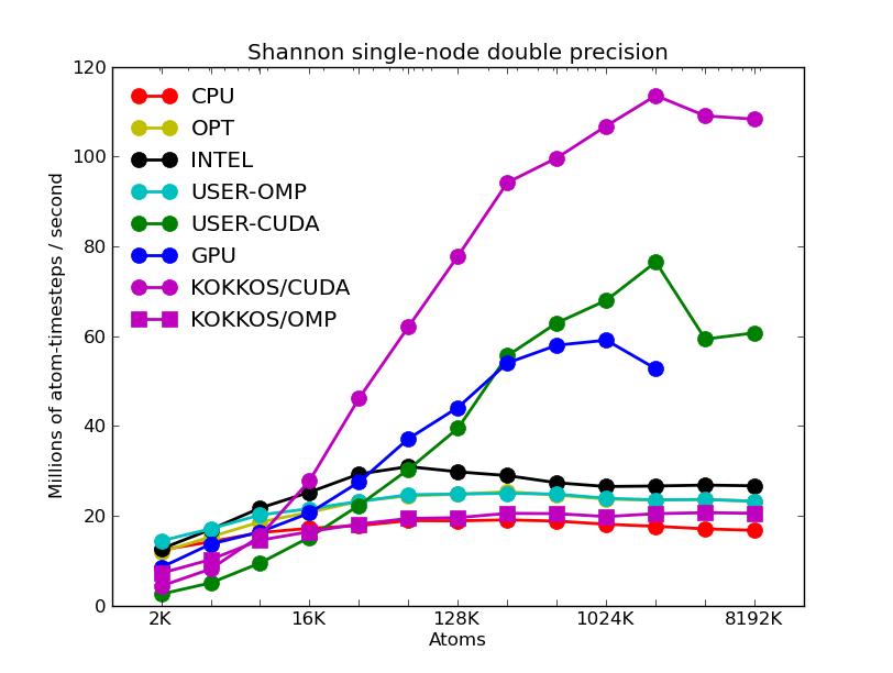
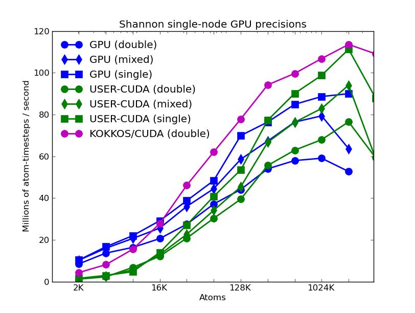
The corresponding raw timing data for the 5 plots is in these 5 files. The 1st column is the x-axis, the 2nd is the time for 100 steps; the 3rd is the y-axis.
The first plot shows the performance of all 6 accelerator packages (two variants for KOKKOS). The GPU, USER-CUDA, and KOKKOS/CUDA curves run primarily on the 2 GPUs. They perform better the more atoms that are modeled. All the other curves run on the 16 CPU cores. All of these performed best using essentially MPI-only parallelization (single thread per MPI task if multi-threading). The CPU curve is for running without enabling any of the accelerator packages. All the runs were in double precision.
The second plot shows the same data as the first (on a different y-axis scale), but only for the runs on the CPU cores. The Intel package has an option to perform pairwise calculations in double, mixed, or single precision, so 3 curves are shown for it.
The third plot also shows the same data as the first, but only for the runs on the GPUs. For each of the 3 packages, runs were made on one or two GPUs. All the runs were in double precision.
The fourth plot shows the performance effect of running the 3 GPU-based packages with varying precision (double, mixed, single). The KOKKOS package only currently allows for double precision calculations.
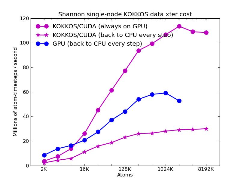
The fifth plot shows the effect on KOKKOS GPU performance of transferring data back and forth between the CPUs and GPUs every timestep. The benchmark problem in the previous 4 plots could run continuously on the GPU (e.g. between occasional thermodynamic output in a production run). But a LAMMPS input script may require more frequent communication back to the CPU. E.g. if a diagnostic is invoked that runs on the CPU or some form of output is triggered every few timesteps. Or if a fix or compute style is used that is not yet KOKKOS-enabled. The benchmark run for this plot required data to move back-and-forth every timestep (worst case). The curve for the GPU package shows this performance hit may be possible to partially overcome, since the GPU package also moves data back and forth every step to perform time integration on the CPU.
The next 2 plots are for parallel runs on 1 to 20 nodes of the cluster. The strong scaling plot is for runs of a 2048K atom problem. The weak scaling plot is for runs with 512K atoms per node. Note that performance (y-axis) is normalized by the number of nodes. Thus in both plots, horizontal lines would be 100% parallel efficiency. Note that for the strong scaling curves on GPUs, there is an pseudo-efficieny loss when running on more nodes due to shrinking the number of atoms per node and thus moving to the left on the single-node GPU performance curves in the plots above.
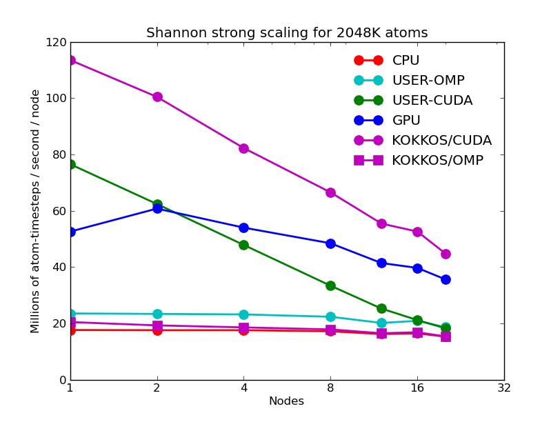
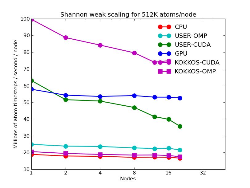
The corresponding raw timing data is in these 2 files. The 1st column is the x-axis, the 2nd is the time for 100 steps; the 3rd is the y-axis.
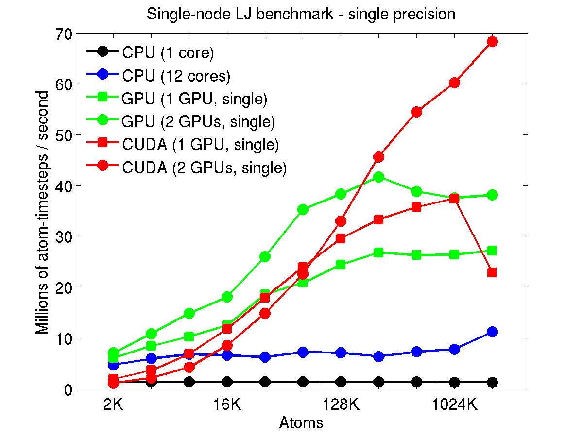
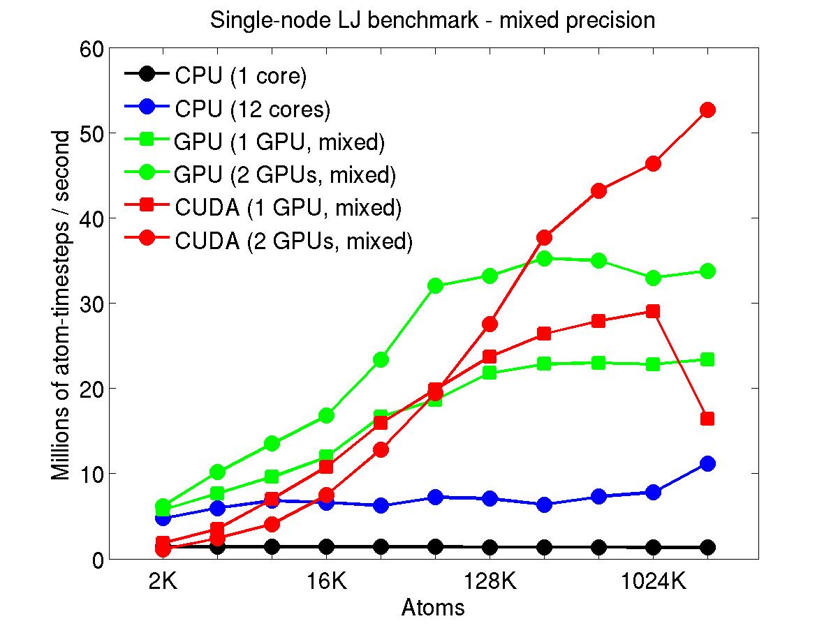
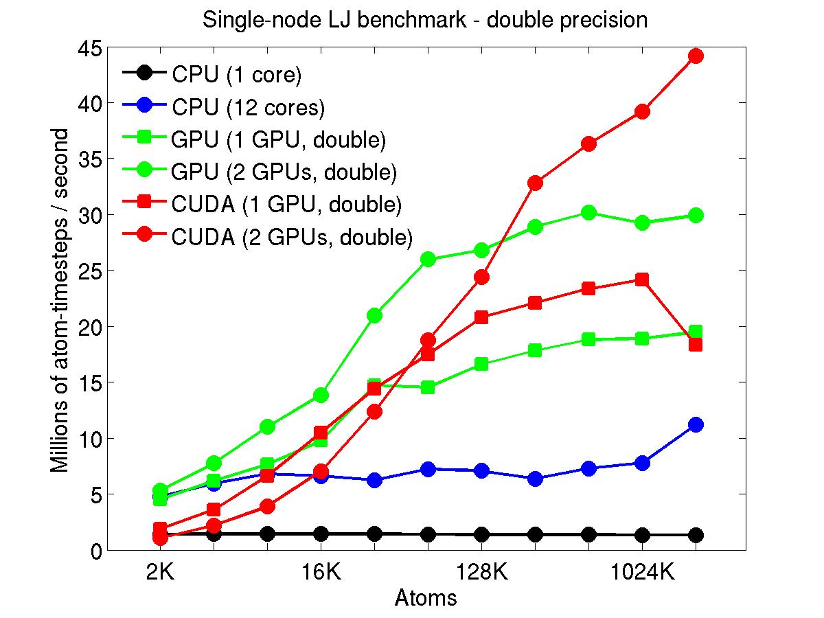
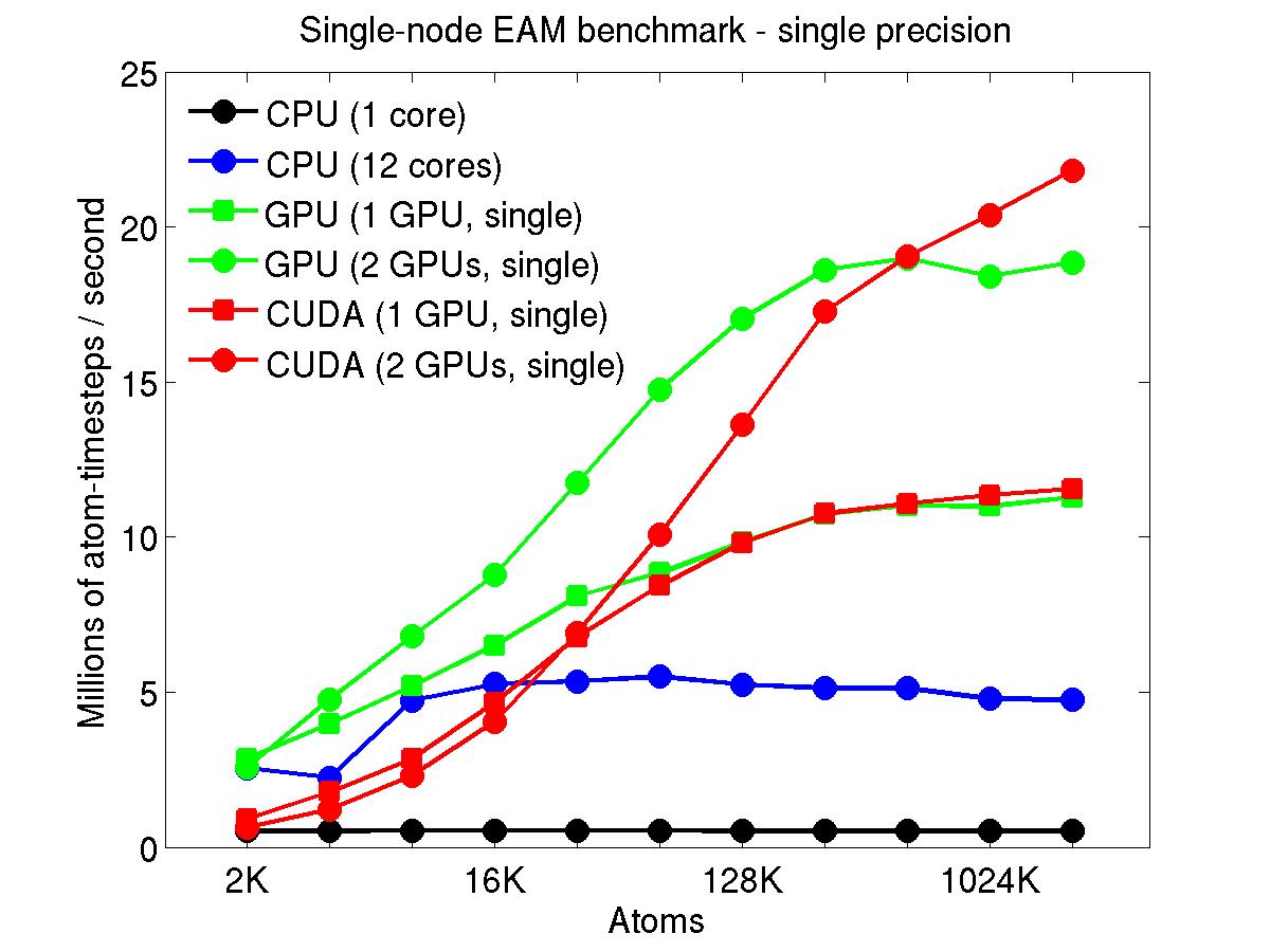
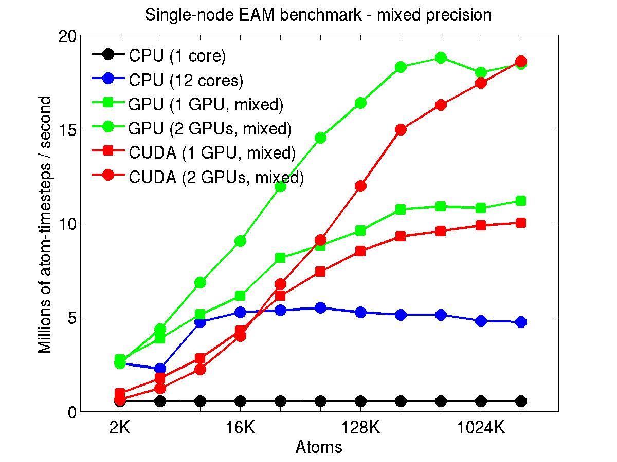
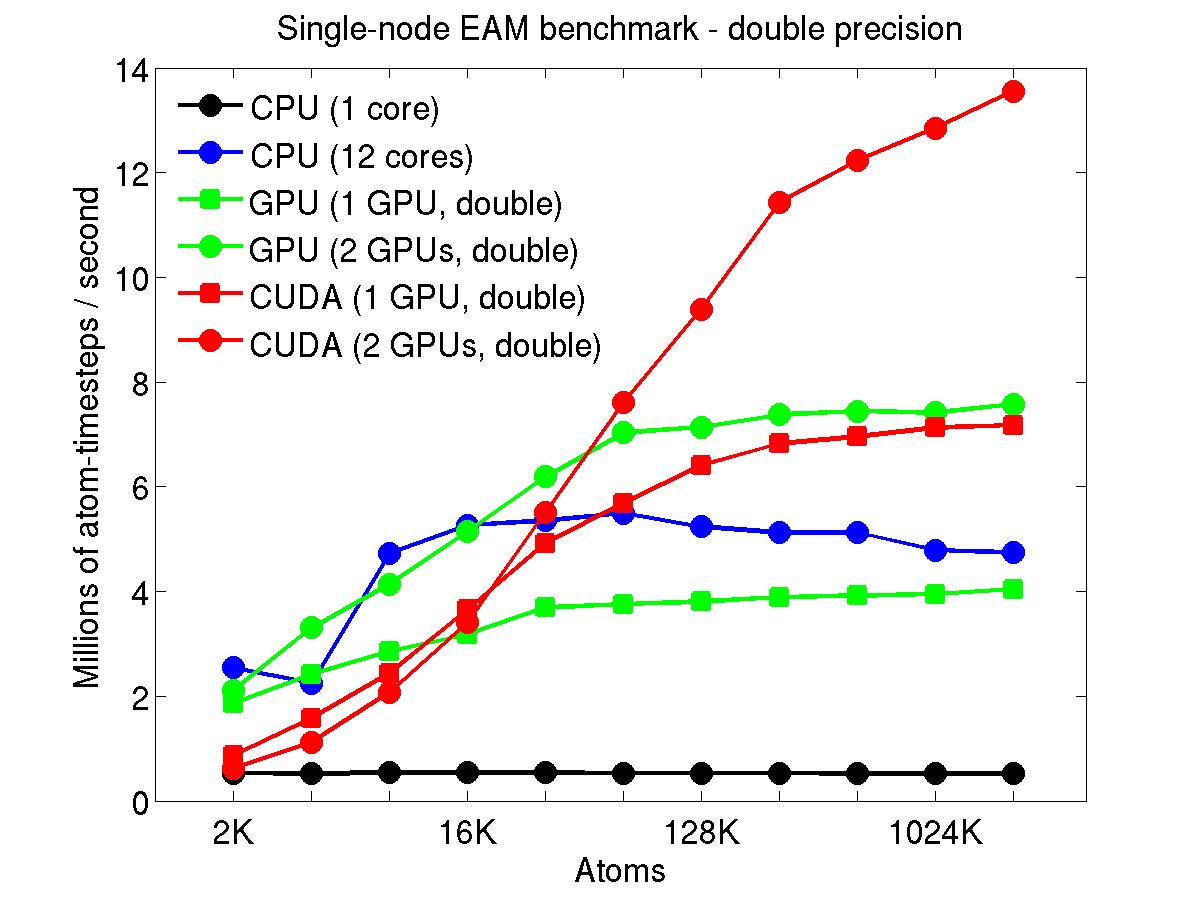
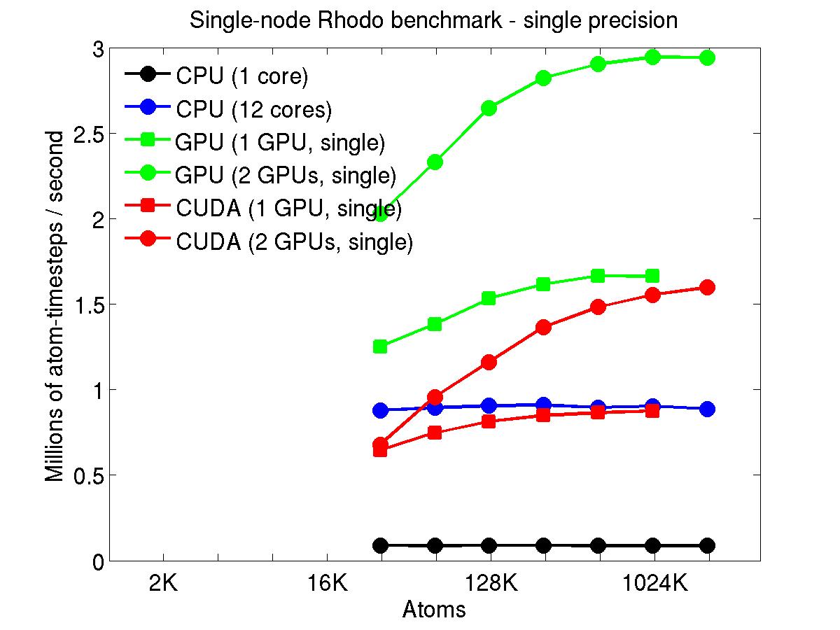
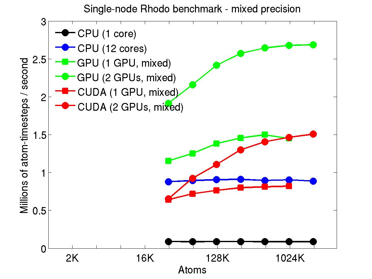
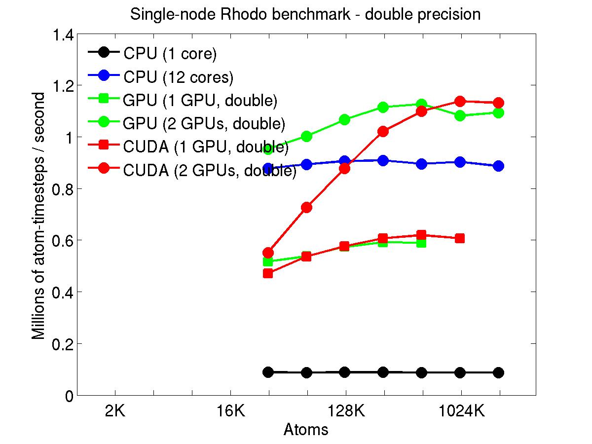
This section shows performance results for a desktop system with dual hex-core Xeon processors and 2 NVIDIA Tesla/Fermi GPUs. More system details are given below, for the "Desktop" entry.
The benchmark problems themselves are described in more detail above in the CPU section. The input scripts and instructions for running these GPU test cases are included in the bench/FERMI directory of the LAMMPS distribution.
The performance is plotted as a function of system size (number of atoms), where the size of the benchmark problems was varied. The Y-axis is atom-timesteps per second. Thus a y-axis value of 10 million for a 1M atom system means it ran at a rate of 10 timesteps/second.
Results are shown for running in CPU-only mode, and on 1 or 2 GPUs, using the GPU package.
The CPU-only results are for running on a single core and on all 12 cores, always in double precision.
For the GPU package, the number of CPU cores/node used was whatever gave the fastest performance for a particular problem size. For small problems this is typically less than all 12; for large problems it is typically all 12. The precision refers to the portion of the calculation performed on the GPU (pairwise interactions). Results are shown for single precision, double precision, and mixed precision which means pairwise interactions calculated in single precision, with the aggregate per-atom force accumulated in double precision.
For the USER-CUDA package, the number of CPU cores used is always equal to the number of GPUs used, i.e. 1 or 2 for this system. The three precisions have the same meaning as for the GPU package, except that other portions of the calculation are also performed on the GPU, e.g. time integration.
Click on the plots for a larger version.
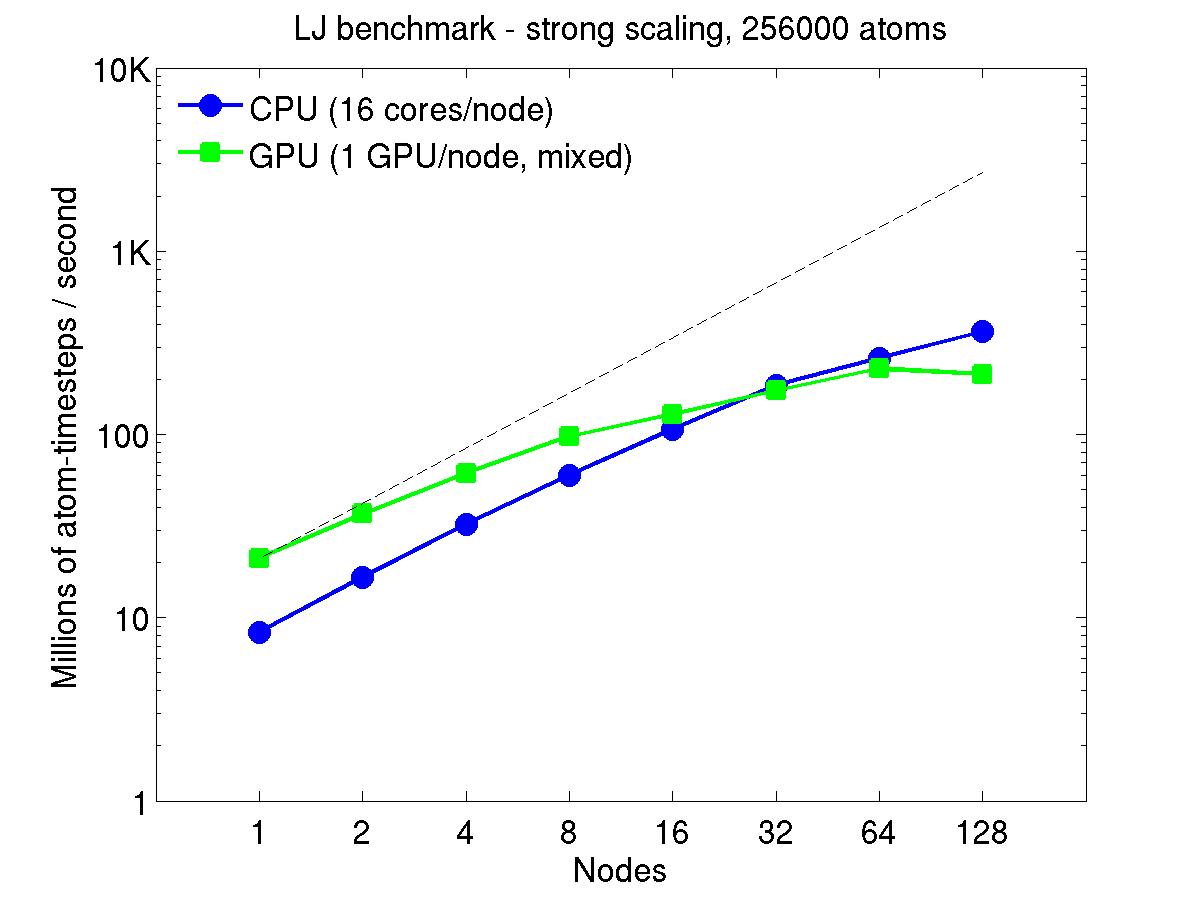
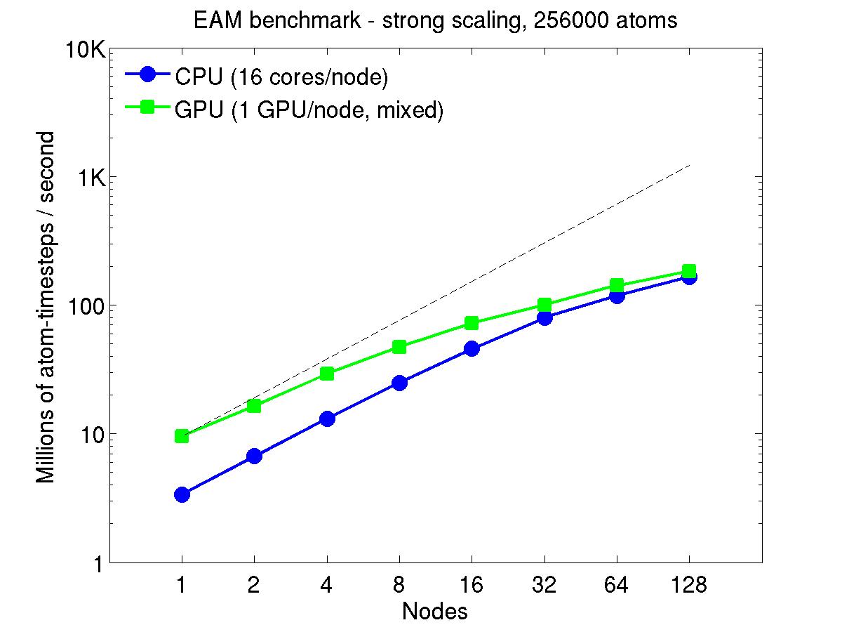
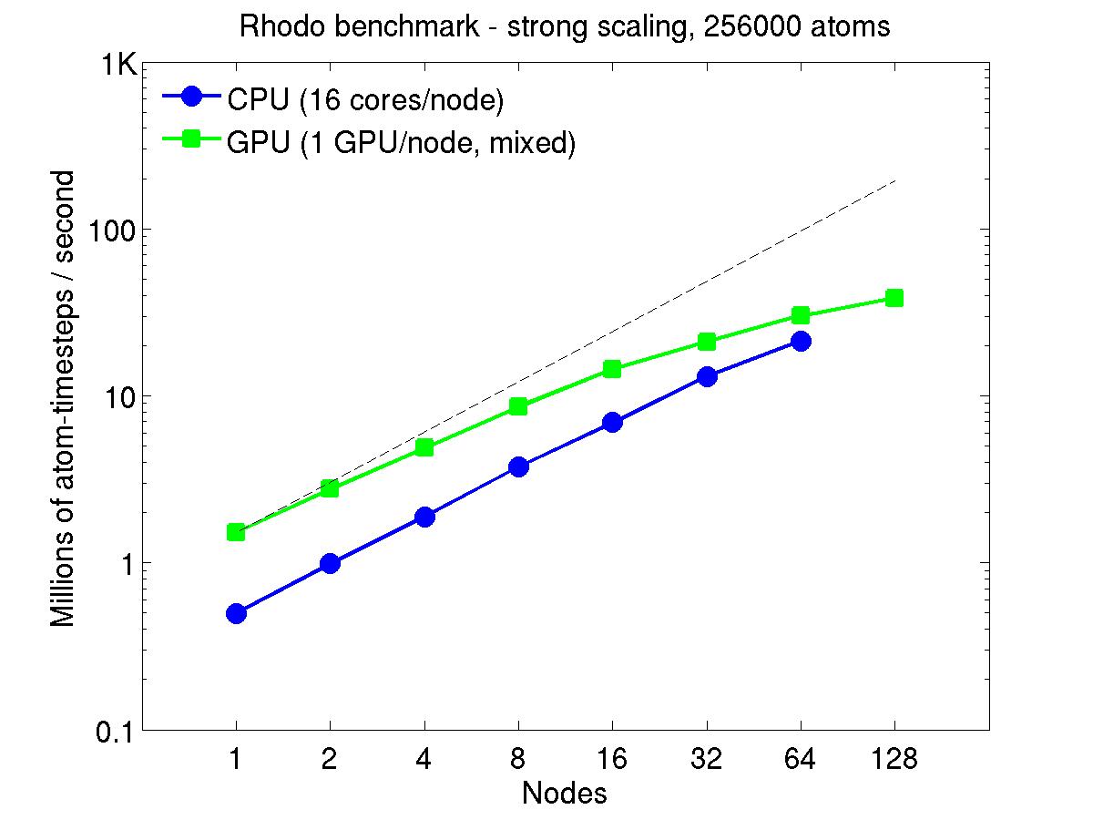
This section shows performance results for the Titan development system, each node of which has a 16-core AMD CPU and a single NVIDIA Tesla/Fermi GPU. More system details are given below, for the "Titan Development" entry. Note that the eventual Titan machine will have Tesla/Kepler GPUs, and more of them.
The benchmark problems themselves are described in more detail above in the CPU section. The input scripts and instructions for running these GPU test cases are included in the bench/FERMI directory of the LAMMPS distribution.
For the rhodopsin benchmark, which computes long-range Coulombics via the PPPM option of the kspace_style command, these benchmarks were run with the run_style verlet/split command, to split the real-space versus K-space computations across the CPUs. This makes little difference on small node counts, but on large node counts, it enables better scaling, since the FFTs computed by PPPM are performed on fewer processors. This was done for both the strong- and weak-scaling results below. The ratio of real-to-kspace processors was chosen to give the best performance, and was 7:1 on this 16 core/node machine.
For the strong-scaling plots, a fixed-size problem of 256,000 atoms was run for all node counts. The node count varied from 1 to 128, or 16 to 2048 cores. The Y-axis is atom-timesteps per second. Thus a value of 10 for the 256,000 atom system means it ran at a rate of roughly 40 timesteps/second.
Strong-scaling results are shown for running in CPU-only mode, and on the GPU, using the GPU package. The CPU-only results are double-precision, the GPU results are for mixed precision which means pairwise interactions calculated in single precision, with the aggregate per-atom force accumulated in double precision. The dotted line indicates the slope for perfect scalability.
For the GPU package, the number of CPU cores/node used was whatever gave the fastest performance for a particular problem size. For the strong-scaling results with the large per-node atom count (256000), this was typically nearly all 16 cores.
Click on the plots for a larger version.
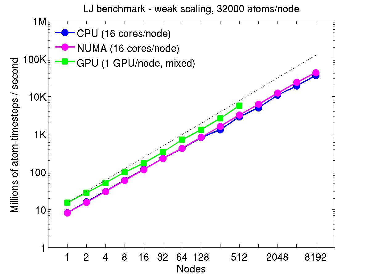
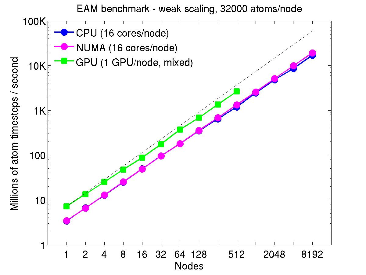
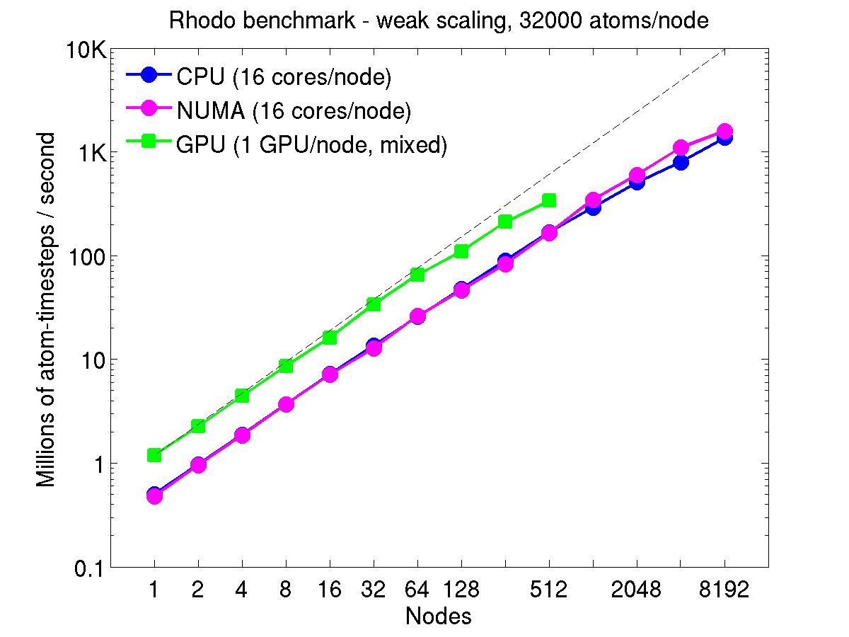
For the weak-scaling plots, a scaled-size problem of 32,000 atoms/node was run for all node counts. The node count varied from 1 to 8192, or 16 to 131072 cores; only 960 nodes on the current development machine have GPUs. Thus the largest system on 8192 nodes has ~262 million atoms.
The Y-axis is atom-timesteps per second. Thus a value of 100 for a 1M atom system (32 nodes) means it ran at a rate of 100 timesteps/second.
Weak-scaling results are shown for running in CPU-only mode, in CPU-only mode with the numa option invoked for the processors command, and on the GPU, using the GPU package. The CPU-only and NUMA results are double-precision, the GPU results are for mixed precision which means pairwise interactions calculated in single precision, with the aggregate per-atom force accumulated in double precision. The dotted line indicates the slope for perfect scalability.
The NUMA results alter the layout of cores to the logical 3d grid of processors that overlays the simulation domain. The processors numa command does this so that cores within a node and within a NUMA region (inside the node) are close together in the topology of the 3d grid, to reduce off-node communication costs. This can give a speed-up of 10-15% on large node counts, as shown in the plots.
For the GPU package, the number of CPU cores/node used was whatever gave the fastest performance for a particular problem size. For the weak-scaling results with the smaller per-node atom count (32000), this was typically 4-8 cores out of 16.
Click on the plots for a larger version.
The following table summarizes the CPU cost of various potentials, as implemented in LAMMPS, each for a system commonly modeled by that potential. The desktop machine these were run on is described below. The last 3 entries are for VASP timings, to give a comparison with DFT calculations. The details for the VASP runs are described below.
The listed timing is CPU seconds per timestep per atom for a one processor (core) run. Note that this is per timestep, as is the ratio to LJ; the timestep size is listed in the table. In each case a short 100-step run of a roughly 32000 atom system was performed. The speed-up is for a 4-processor run of the same 32000-atom system. Speed-ups greater than 4x are due to cache effects.
To first order, the CPU and memory cost for simulations with all these potentials scales linearly with the number of atoms N, and inversely with the number of processors P when running in parallel. This assumes the density doesn't change so that the neighbors per atom stays constant as you change N. This holds for N/P ratios larger than some threshhold, say 1000 atoms per processor. Thus you can use this data to estimate the run-time of different size problems on varying numbers of processors.
| Potential | System | # Atoms | Timestep | Neighs/atom | Memory | CPU | LJ Ratio | P=4 Speed-up | Input script | Tarball |
| Granular | chute flow | 32000 | 0.0001 tau | 7.2 | 33 Mb | 2.08e-7 | 0.26x | 4.28x | in.granular | bench_granular.tar.gz |
| FENE bead/spring | polymer melt | 32000 | 0.012 tau | 9.7 | 8.4 Mb | 2.86e-7 | 0.36x | 3.78x | in.fene | bench_fene.tar.gz |
| Lennard-Jones | LJ liquid | 32000 | 0.005 tau | 76.9 | 12 Mb | 8.01e-7 | 1.0x | 3.56x | in.lj | bench_lj.tar.gz |
| DPD | pure solvent | 32000 | 0.04 tau | 41.3 | 9.4 Mb | 1.22e-6 | 1.53x | 3.54x | in.dpd | bench_dpd.tar.gz |
| EAM | bulk Cu | 32000 | 5 fmsec | 75.5 | 13 Mb | 1.87e-6 | 2.34x | 3.83x | in.eam | bench_eam.tar.gz |
| REBO | polyethylene | 32640 | 0.5 fmsec | 149 | 33 Mb | 3.18e-6 | 3.97x | 3.61x | in.rebo | bench_rebo.tar.gz |
| Stillinger-Weber | bulk Si | 32000 | 1 fmsec | 30.0 | 11 Mb | 3.28e-6 | 4.10x | 3.83x | in.sw | bench_sw.tar.gz |
| Tersoff | bulk Si | 32000 | 1 fmsec | 16.6 | 9.2 Mb | 3.74e-6 | 4.67x | 3.92x | in.tersoff | bench_tersoff.tar.gz |
| ADP | bulk Ni | 32000 | 5 fmsec | 83.6 | 25 Mb | 5.58e-6 | 6.97x | 3.61x | in.adp | bench_adp.tar.gz |
| EIM | crystalline NaCl | 32000 | 0.5 fmsec | 98.9 | 14 Mb | 5.60e-6 | 6.99x | 3.86x | in.eim | bench_eim.tar.gz |
| Peridynamics | glass fracture | 32000 | 22.2 nsec | 422 | 144 Mb | 7.46e-6 | 9.31x | 3.78x | in.peri | bench_peri.tar.gz |
| SPC/E | liquid water | 36000 | 2 fmsec | 700 | 86 Mb | 8.77e-6 | 11.0x | 3.46x | in.spce | bench_spce.tar.gz |
| CHARMM + PPPM | solvated protein | 32000 | 2 fmsec | 376 | 124 Mb | 1.13e-5 | 14.1x | 3.66x | in.protein | bench_protein.tar.gz |
| MEAM | bulk Ni | 32000 | 5 fmsec | 48.8 | 54 Mb | 1.32e-5 | 16.5x | 3.73x | in.meam | bench_meam.tar.gz |
| Gay-Berne | ellipsoid mixture | 32768 | 0.002 tau | 140 | 21 Mb | 2.20e-5 | 27.5x | 3.63x | in.gb | bench_gb.tar.gz |
| BOP | bulk CdTe | 32000 | 1 fmsec | 4.4 | 74 Mb | 2.51e-5 | 31.3x | 3.88x | in.bop | bench_bop.tar.gz |
| AIREBO | polyethylene | 32640 | 0.5 fmsec | 681 | 101 Mb | 3.25e-5 | 40.6x | 3.66x | in.airebo | bench_airebo.tar.gz |
| ReaxFF/C | PETN crystal | 32480 | 0.1 fmsec | 667 | 976 Mb | 1.09e-4 | 136x | 3.17x | in.reaxc | bench_reaxc.tar.gz |
| COMB | crystalline SiO2 | 32400 | 0.2 fmsec | 572 | 85 Mb | 2.00e-4 | 250x | 3.89x | in.comb | bench_comb.tar.gz |
| eFF | H plasma | 32000 | 0.001 fmsec | 5066 | 365 Mb | 2.16e-4 | 270x | 3.71x | in.eff | bench_eff.tar.gz |
| ReaxFF | PETN crystal | 16240 | 0.1 fmsec | 667 | 425 Mb | 2.84e-4 | 354x | 3.78x | in.reax | bench_reax.tar.gz |
| VASP/small | water | 192/512 | 0.3 fmsec | N/A | 320 procs | 26.2 | 17.7e6 | 100% | N/A | N/A |
| VASP/medium | CO2 | 192/1024 | 0.8 fmsec | N/A | 384 procs | 252 | 170e6 | 100% | N/A | N/A |
| VASP/large | Xe | 432/3456 | 2.0 fmsec | N/A | 384 procs | 1344 | 908e6 | 100% | N/A | N/A |
Notes:
Details for different systems:
The Lennard-Jones benchmark problem described above (100 timesteps, reduced density of 0.8442, 2.5 sigma cutoff, etc) has been run on different machines for billion-atom tests. For the LJ benchmark LAMMPS requires a little less than 1/2 Terabyte of memory per billion atoms, which is used mostly for neighbor lists.
| Machine | # of Atoms | Processors | CPU Time (secs) | Parallel Efficiency | Flop Rate | Date |
| Keeneland | 1 million | 1 GPU | 2.35 | 100% | 27.0 Gflop | 2012 |
| Keeneland | 1 billion | 288 GPUs | 17.7 | 46.3% | 3.60 Tflop | 2012 |
| Lincoln | 1 million | 1 GPU | 4.24 | 100% | 15.0 Gflop | 2011 |
| Lincoln | 1 billion | 288 GPUs | 28.7 | 51.3% | 2.21 Tflop | 2011 |
| Cray XT5 | 1 million | 1 | 148.7 | 100% | 427 Mflop | 2011 |
| Cray XT5 | 1 billion | 1920 | 103.0 | 75.1% | 616 Gflop | 2011 |
| Cray XT3 | 1 million | 1 | 235.3 | 100% | 270 MFlop | 2006 |
| Cray XT3 | 1 billion | 10000 | 25.1 | 93.6% | 2.53 Tflop | 2006 |
| Cray XT3 | 10 billion | 10000 | 246.8 | 95.2% | 2.57 Tflop | 2006 |
| Cray XT3 | 40 billion | 10000 | 979.0 | 96.0% | 2.59 Tflop | 2006 |
| IBM BG/L | 1 million | 1 | 898.3 | 100% | 70.7 Mflop | 2005 |
| IBM BG/L | 1 billion | 4096 | 227.6 | 96.3% | 279 Gflop | 2005 |
| IBM BG/L | 1 billion | 32K | 30.2 | 90.7% | 2.10 Tflop | 2005 |
| IBM BG/L | 1 billion | 64K | 16.0 | 85.6% | 3.97 Tflop | 2005 |
| IBM BG/L | 10 billion | 64K | 148.9 | 92.0% | 4.26 Tflop | 2005 |
| IBM BG/L | 40 billion | 64K | 585.4 | 93.6% | 4.34 Tflop | 2005 |
| ASCI Red | 32000 | 1 | 62.88 | 100% | 32.3 Mflop | 2004 |
| ASCI Red | 750 million | 1500 | 1156 | 85.0% | 41.2 Gflop | 2004 |
The parallel efficiencies are estimated from the per-atom CPU or GPU time for a large single processor (or GPU) run on each machine:
The aggregate flop rate is estimated using the following values for the pairwise interactions, which dominate the run time:
This is a conservative estimate in the sense that flops computed for atom pairs outside the force cutoff, building neighbor lists, and time integration are not counted. For the USER-CUDA package running on GPUs, Newton's 3rd law is not used (because it's faster not to), which doubles the pairwise interaction count, but that is not included in the flop rate either.
This section lists characteristics of machines used in the benchmarking along with options used in compiling LAMMPS. The communication parameters are for bandwidth and latency at the MPI level, i.e. what a program like LAMMPS sees.
Desktop = Dell Precision T7500 desktop workstation running Red Hat linux
Mac laptop = PowerBook G4 running OS X 10.3
ASCI Red = ASCI Intel Tflops MPP
Ross = CPlant DEC Alpha/Myrinet cluster
Liberty = Intel/Myrinet cluster packaged by HP
Cheetah = IBM p690 cluster
Xeon/Myrinet cluster = Spirit
IBM p690+ cluster = HPCx
IBM BG/L = Blue Gene Light
Cray XT3 = Red Storm
Cray XT5 = xtp
Lincoln = GPU cluster
Keeneland = GPU cluster
Titan Development = GPU-enabled supercomputer (used to be Jaguar)